__Topic \#3__ __Data __ __analysis__  __Fiddling__ __ __ __with__ __ __ __signals__ __ __ __and__ __ __ __frequencies__ sampling\, frequency space representations\, filters and filter properties\, convolution theorem __Spectral__ __ __ __analysis__ \(windowed\) Fourier\, Hilbert\, wavelets\, coherence measures __Multidimensional __ __representations__ PCA\, ICA\, SVD\, k\-means __Classification__ ROC\, k\-NN\, SVM __Fiddling__ __ __ __with__ __ __ __signals__ __ __ __and__ __ __ __frequencies__ frequency above Nyquist __Sampling__ Sampled signals have a limited time resolution and a limited range and precision 2 bits range = 4 states __Reminder__ __: __ __the__ __ Fourier __ __transform__ __Signals s\(t\)__ can also be represented in Fourier space as __complex__ __ __ __coefficients__ __ S\(f\)__ \. Transform forth and back by \(inverse\) __Fourier __ __transform__ \. Visualize a Fourier\-transformed signal as __power __ __spectral__ __ __ __density__ \(remember lecture/exercise in Theo\. 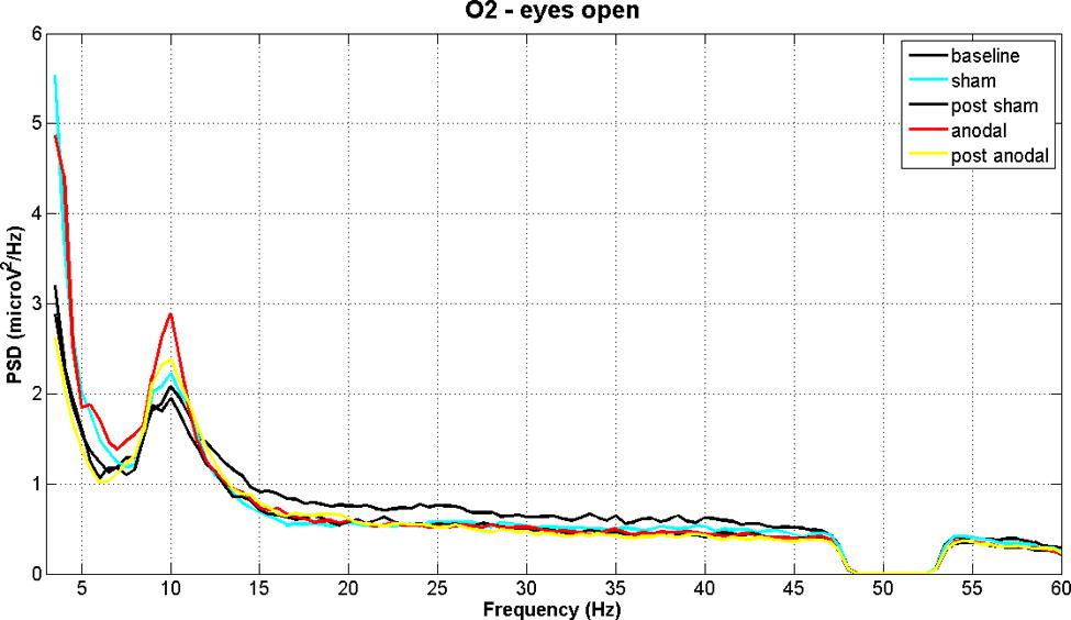Neurosciences\):  some interesting signal feature at f=10 Hz …there‘s a hole in the bucket\, dear Liza\, dear Liza\! _https://en\.wikipedia\.org/wiki/There%27s\_a\_Hole\_in\_My\_Bucket_ _source_ _: neuroimage\.usc\.edu_ __How__ __ __ __can__ __ __ __we__ __ __ __extract__ __ __ __signals__ __ at __ __frequency__ __ __ __ranges__ __ __ __of__ __ __ __interest__ __\, __ __or__ __ __ __put__ __ __ __holes__ __ in __ __the__ __ __ __spectrum__ __ __ __of__ __ __ __the__ __ __ __data__ __?__  Visualizing in frequency space what a filter does… amplitude drops to ~70%  _https://www\.allaboutcircuits\.com/technical\-articles/an\-introduction\-to\-filters/_ __Quality __ __factor__ : __Q=f0/\(f2\-f1\)__ __dB = __ __decibel__ __: __ defined as __10 log\(P2/P1\) dB __ for __power __ __ratio__ P2 vs\. P1 …therefore\, __20 log\(A2/A1\) dB __ for __amplitude__ __ __ __ratios__ \! \(note that mathematical „log“ is numpyically „log10“\!\) __Filter __ __order__ : __~ __ __slope__ __ __ __of__ __ __ __decay__  __Filtering__ __ __ __with__ __ Python__ We like the butterworth filter provided by the __scipy\.signal__ __ __ module\. 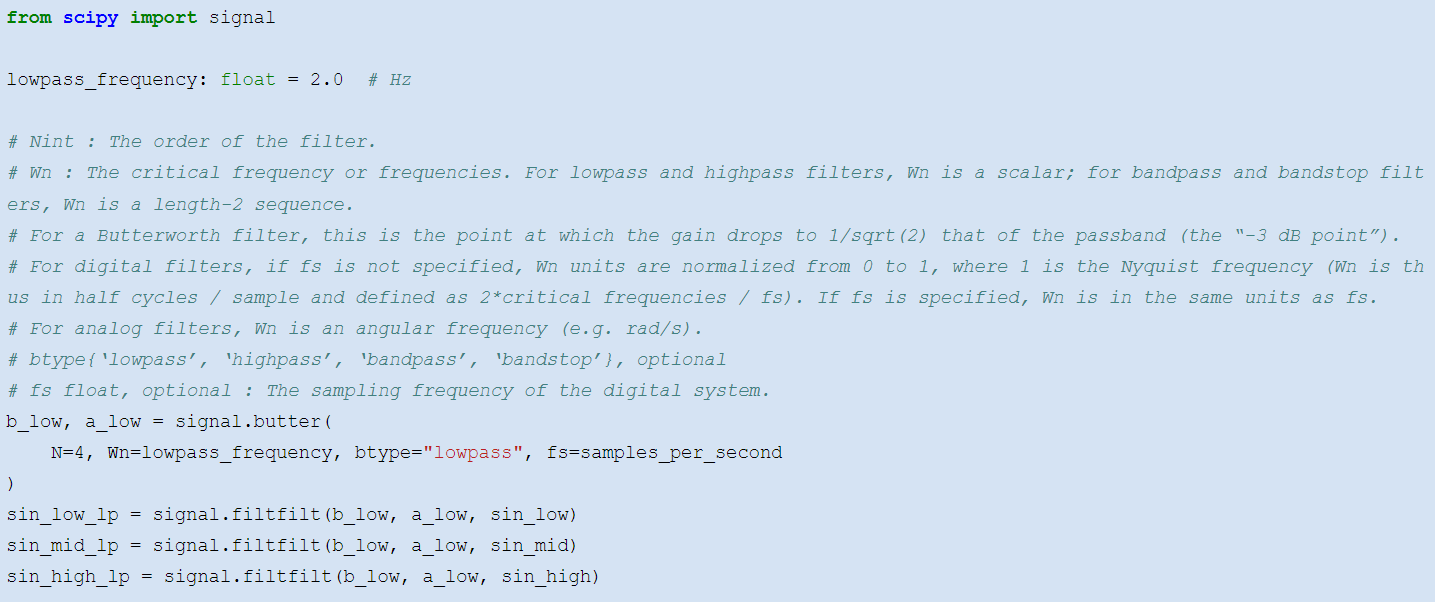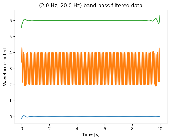One uses __butter__ to construct the filter\, and __filtfilt__ to apply the constructed filter to a time series:  __Sample __ __signals__ __ __ __used__ __ in __ __the__ __ __ __following__ __ __ __slides__ __:__     __High\-pass __ __and__ __ __ __bandpass__    __beware__ __\!__ __transients__ __\!__  Filters imply phase shifts\. To compensate\, combine for\- and backward filtering\. Filter first before downsampling \(see example\)\. To inspect a filter\, filter a white noise signal and plot PSD\. Take care\, transients at start and end of signal The more parameter you specify\, the more difficult is it to design a filter __blue__ __: __ original signal \, sampled at 2500 Hz __red__ __: __ downsampled to 25 Hz __black__ __: __ first filtered\, then downsampled to 25 Hz The convolution theorem states that in Fourier space \, convolutions are expressed by multiplication of the transformed signal and filter \. If you transform a filter into Fourier space\, you can investigate its properties by considering it a ‚mask‘ for your time series representation\. You can use the convolution theorem to perform convolutions efficiently \, using FFT\. __Example__ __: __ __low__ __\-pass __ __filter__ __More __ __information__ __:__ [https://davrot\.github\.io/pytutorial/scipy/scipy\.signal\_butterworth](https://davrot.github.io/pytutorial/scipy/scipy.signal_butterworth/) [/](https://davrot.github.io/pytutorial/scipy/scipy.signal_butterworth/) __Spectral__ __ __ __analysis__ __ __ __ANDA __ __tutorial__ __…__ Switch presentations __Wavelet Transform in Python__ One can use the __pywt__ module\, and requires essentially only two commands for creating a ‚mother wavelet‘ and applying it to the time series of interest: \# The wavelet we want to use\.\.\. mother = pywt \.ContinuousWavelet \( "cmor1\.5\-1\.0" \) \# \.\.\.applied with the parameters we want: complex\_spectrum \, frequency\_axis = pywt \. cwt \(     data = test\_data \, scales = wave\_scales \, wavelet = mother \, sampling\_period = dt \) However\, working with the wavelet transform requires to think about the scales or frequency bands\, their spacing\, proper definition of time/frequency resolution\, taking care of the cone\-of\-interest etc… Full code at: [https://davrot\.github\.io/pytutorial/pywavelet](https://davrot.github.io/pytutorial/pywavelet/)[/](https://davrot.github.io/pytutorial/pywavelet/) __More __ __information__ __:__ [https://davrot\.github\.io/pytutorial/pywavelet](https://davrot.github.io/pytutorial/pywavelet/) [/](https://davrot.github.io/pytutorial/pywavelet/) __Multidimensional __ __representations__ Neural recordings often yield a large number of signals xi\(t\)\. Typically\, these signals contain a mixture of \(internal and external\) sources sj\(t\)\. __Example__ __: __ One EEG signal contains the activity of millions of neurons\. __Goal: __ find the neural sources s\(t\) contained in the signals x\(t\) __Also:__ Assessment of dimensionality of a representation Dimensionality reduction\. Get the principal components\. Remove common sources \(common reference\, line noise\, heartbeat artifacts\, etc\.\) … __PCA – __ __principal__ __ __ __component__ __ __ __analysis__ Find sources which are uncorrelated with each other \. Uncorrelated means that the source vectors S will be orthogonal to each other \. PCA finds matrix WPCA such that X is explained by X = S WPCA\.  remove mean? remove std? 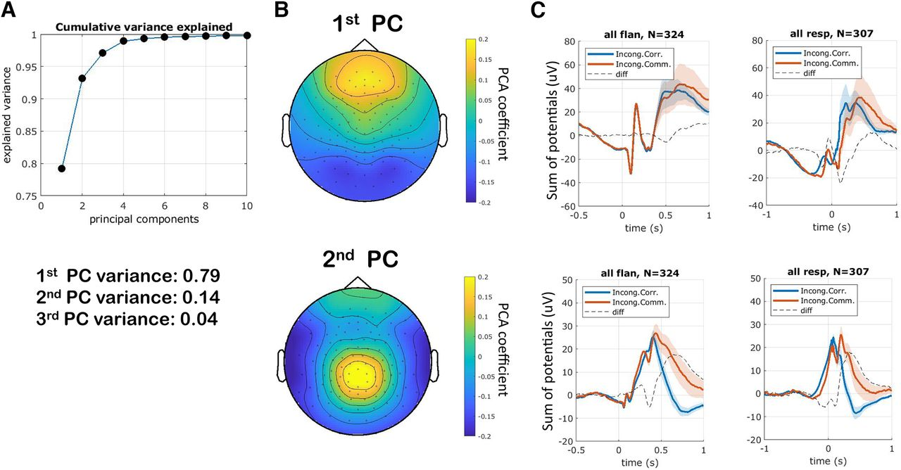W PCA \-1 = W PCA T \, so S = X W PCA T __Example__ __: n __ __signals__ __ __ __of__ __ __ __duration__ __ t: __ S: \(t x n\) – n source vectors WPCA: \(n x n\) – mixture matrix X: \(t x n\) – n observation vectors __Visualization__ __:__ W PCA \[k\, :\] shows how the k\- th component contributes to the n observations :   __PCA – __ __principal__ __ __ __component__ __ __ __analysis__ __: Python__ Use __class__ __ PCA __ from __sklearn\.decomposition__ module:  After defining an instance\, you can use __fit__ for fitting a transform\, and __transform__ for transforming X to S\. __fit\_transform__ combines these steps\, and __inverse\_transform__ __ __ does the transfrom from S to X\. The attribute __components__ __\___ will contain the PCA transformation components Components will be sorted with descending \( explained \) variance \. from sklearn \. decomposition import PCA \# transform x to s pca = PCA \(\) s = pca \. fit\_transform \( x \) w\_pca = pca \. components \_ \# transform s to x x\_recover = pca\. inverse\_transform \(s\) also\_x\_recover = s@w\_pca W PCA \-1 = W PCA T \, so S = X W PCA T __Take care\! __ __Instead__ __ __ __of__ __ X __ __= S __ __W__ __PCA__ __\, __ __the__ __ __ __transform__ __ __ __is__ __ also __ __often__ __ __ __defined__ __ __ __as__ __ X‘ __ __= __ __W__ __PCA__ __ S‘\. This __ __makes__ __ X‘\, S‘ \(n x t\) __ __instead__ __ __ __of__ __ \(t x n\) __ __matrices__ __\!__ __SVD – Singular Value __ __Decomposition__ The singular value decomposition decmposes a matrix __M__ into two unitary matrices U and V\, and a diagonal matrix ∑: __M = U__ __ __ __∑ V\* __ Assumptions are UTU = UUT = I\, and VTV = VVT = I with I being the unit matrix\.  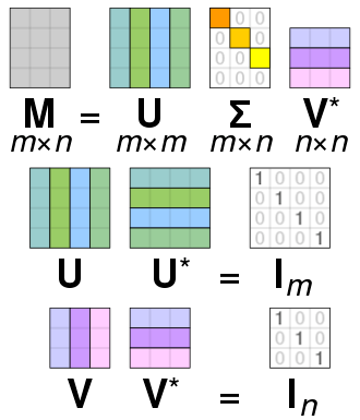__Relation __ __to__ __ PCA: __ Consider m denotes ‚time‘ t\,and n <=t\. Then M are the observations X\, V\* will be WPCA\, and S = U ∑ the uncorrelated principal components\, related via: __X = S W__ __PCA__ \. __ICA – __ __independent__ __ __ __component__ __ __ __analysis__ ICA assumes also a linear mixture of ‚ sources ‘ via X = S W ICA \. However\, here the goal is to find sources which are statistically independent to each other\. __The ICA __ __transform__ __ __ __is__ __ not __ __unique__ __ __ __and__ __ __ __depends__ __ on __ __the__ __ __ __independence__ __ __ __criterion__ __\!__ remove mean? remove std? is STS trivially diagonal?  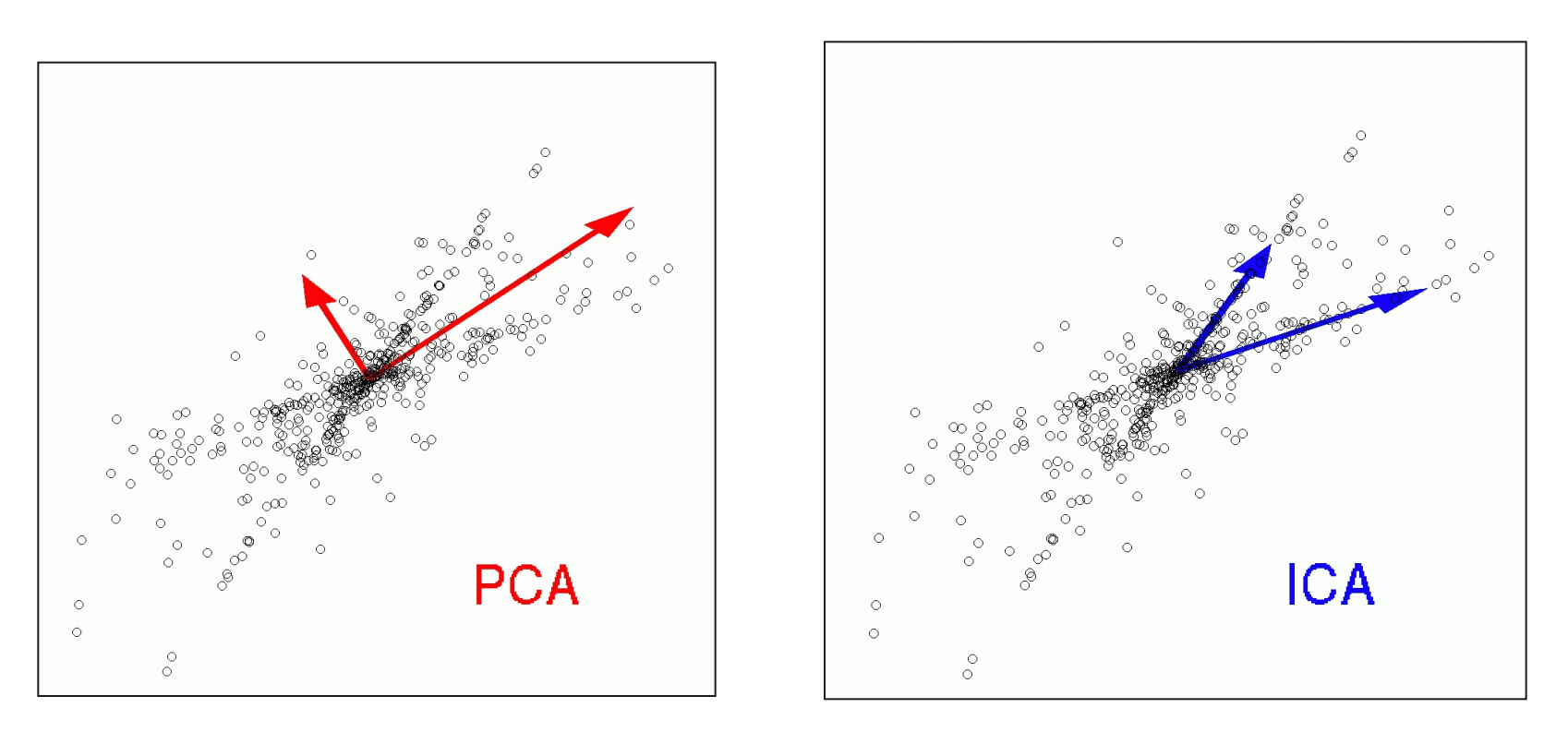When might ICA be more appropriate than PCA? __Example__ __:__ __ __ __Independence __ __criteria__ __:__ minimization of mutual information maximization of non\-Gaussianity __ICA – __ __independent__ __ __ __component__ __ __ __analysis__ __: Python__ Use __class__ __ __ __FastICA__ __ __ from __sklearn\.decomposition__ module\. The usage is very similar to __PCA__ \. from sklearn \. decomposition import FastICA \# transform x to s ica = FastICA \(\) s = ica \. fit\_transform \( x \) w\_ica = ica \. components \_ \# transform s to x x\_recover = ica \. inverse\_transform \( s \) remove mean? remove std? is STS trivially diagonal?  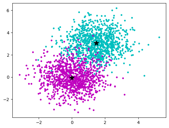We have __multidimensional __ __samples__ __ X__ and expect that they stem from different ‚classes‘\, e\.g\. spike waveforms where spikes from one particular cell constitute one class\. 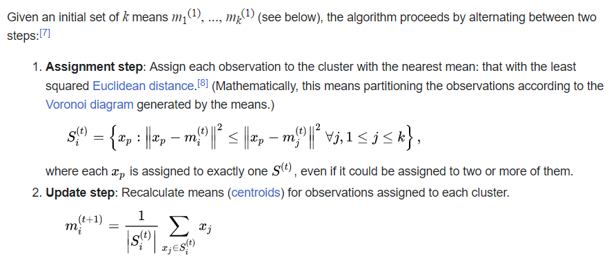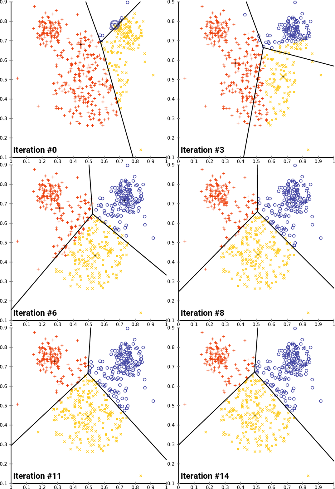Samples from a particular class should have smaller distance than samples stemming from different classes: __The k\-__ __means__ __ Clustering __ __Algorithm__  _description_ _ _ _and_ _ _ _animation_ _ _ _from_ _ Wikipedia_  __cluster\_centers__ __\___  __The k\-__ __means__ __ Clustering __ __Algorithm__ __: Python__   __More __ __information__ __:__ [https://davrot\.github\.io/pytutorial/scikit\-learn/overview](https://davrot.github.io/pytutorial/scikit-learn/overview/) [/](https://davrot.github.io/pytutorial/scikit-learn/overview/) [https://davrot\.github\.io/pytutorial/scikit\-learn/pca](https://davrot.github.io/pytutorial/scikit-learn/pca/) [/](https://davrot.github.io/pytutorial/scikit-learn/pca/) [https://davrot\.github\.io/pytutorial/scikit\-learn/fast\_ica](https://davrot.github.io/pytutorial/scikit-learn/fast_ica/) [/](https://davrot.github.io/pytutorial/scikit-learn/fast_ica/) [https://davrot\.github\.io/pytutorial/scikit\-learn/kmeans](https://davrot.github.io/pytutorial/scikit-learn/kmeans/) [/](https://davrot.github.io/pytutorial/scikit-learn/kmeans/) __Classification__ __ __ __yields__ __ __ __information__ __ __ __about__ __ __ __information__ __ in __ __data__ __…__ __Receiver\-operator\-__ __characteristics__ __ \(ROC\): __ a simple tool for quick inspection for both simple and complex data sets __K\-__ __nearest__ __\-__ __neighbor__ __ __ __classifier__ __ \(__ __kNN__ __\): __ easy to implement\, suited for a quick inspection __Support __ __vector__ __ __ __machine__ __ \(SVM\): __ an almost state\-of\-the\-art tool for \(non\-\)linear classification of large data sets\. Very useful if you don‘t want to fire up your deep network and NVidia GPU for every almost trivial problem… __Important__ __: __ For classification \, you need a __training__ __ __ __data__ __ __ __set__ \, and a __test__ __ __ __data__ __ __ __set__ \. Each data set contains \(a large number of \) __samples__ together with their __labels__ \. You are __not __ __allowed__ __ __ __to__ __ __ __use__ __ __ __the__ __ __ __test__ __ __ __set__ __ __ __for__ __ __ __training__ \.  __Receiver\-Operator __ __Characteristics__ The situation: one recorded signal r\, two potential causes „\+“ or „\-“: __radio__ __ __ __signal__ __ r=__ __enemy__ __ __ __plane __ __\(\-\) __ __or__ __ __ __swarm__ __ __ __of__ __ __ __birds__ __ \(\+\)?__ __How__ __ __ __can__ __ __ __we__ __ __ __distinguish__ __ __ __between__ __ „\+“ __ __and__ __ „\-“?__ Simplest estimator: use threshold z\, if sample r0 is smaller than z\, attribute to „\-“\, otherwise to „\+“ Can we find an __optimal z__ ? Yes\, the idea is to plot the __true__ __ positives \(__ __β__ __\) __ against the __false__ __ positives \(__ __α__ __\)__ while changing z \(ROC curve\)\. Classification accuracy has a __maximum__ __/__ __minimum__ __ __ __when__ __ __ __the__ __ __ __rates__ __ __ __of__ __ __ __change__ __ __ __are__ __ __ __equal__ __ __ __\(__ __slope__ __=1\)__ \. __Summary: __ __ROC'n'Roll__ …it‘s a nice tool for quick inspection how well a scalar variable allows to discriminate between two situations\! 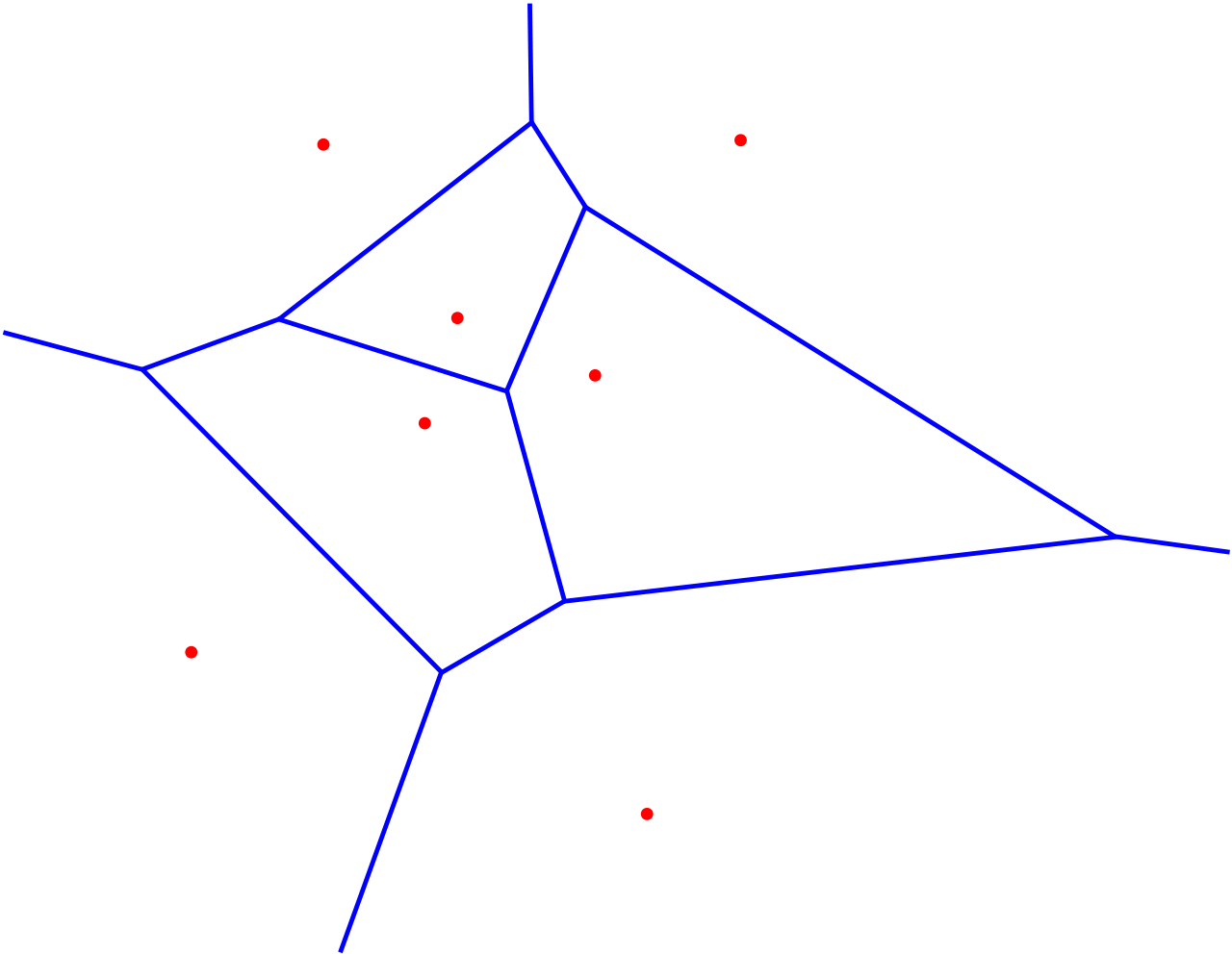__What's wrong if the ROC curve is under the diagonal?__ __Discriminability__ __: __ difference of means relative to std: d‘ := \(r\+\-r\- \)/ σ __k\-__ __Nearest__ __\-__ __Neighbour__ __ __ __Classifier__ __:__  Super\-easy to explain\, super\-easy to implement\, super memory consuming\! The __x__ __i__ are samples of the training data set with labels __y__ __i__ \. Every sample from the test data set __inside__ __ __ __the__ __ __ __neighborhood__ __ __ __of__ __ x__ __42__ __ \(__ __Voronoi__ __ __ __cell__ __\) __ gets assigned the label __y__ __42__ \(k=1\)… …or the majority vote/mixture of the __labels__ __ __ __of__ __ __ __the__ __ k __ __nearest__ __ __ __neighbors__ \. __The __ __support__ __ __ __vector__ __ __ __machine__ __ \(SVM\)__ You know how a simple perceptron works \(lecture Theoretical Neurosciences\)? The SVM is doing the same thing\, but __transforms__ __ __ __the__ __ __ __data__ __ __ __into__ __ a __ __higher__ __\-dimensional __ __space__ before it performs a __linear __ __classification__ __ __ __by__ __ __ __using__ __ an __ __appropriately__ __ __ __placed__ __ __ __separating__ __ hyperplane__ :  __separating__ __hyperplane__ __Python __ __tools__ __ __ __for__ __ __ __elementary__ __ __ __classification__ __ __ __tasks__ __:__ __ROC__ and __kNN__ – easy to code on your own \(and a good training for you\!\)…  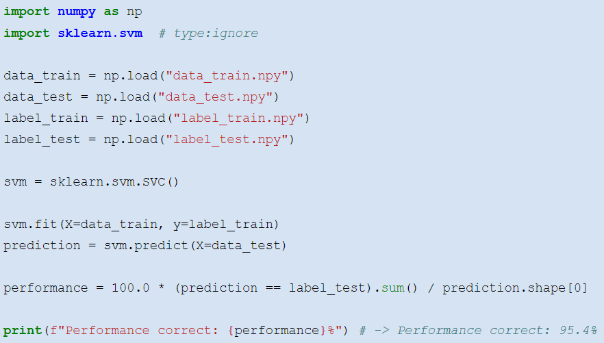Learning an __SVM__ is more tricky\. __scikit\-learn__ provides you with a good tool: __More __ __information__ __:__ [https://davrot\.github\.io/pytutorial/numpy/roc](https://davrot.github.io/pytutorial/numpy/roc/) [/](https://davrot.github.io/pytutorial/numpy/roc/) [https://davrot\.github\.io/pytutorial/numpy/knn](https://davrot.github.io/pytutorial/numpy/knn/) [/](https://davrot.github.io/pytutorial/numpy/knn/) [https://davrot\.github\.io/pytutorial/scikit\-learn/svm](https://davrot.github.io/pytutorial/scikit-learn/svm/) [/](https://davrot.github.io/pytutorial/scikit-learn/svm/)