35 KiB
Topic #3 __Data __ analysis
Fiddling __ __ with __ __ signals __ __ and __ __ frequencies
sampling, frequency space representations, filters and filter properties, convolution theorem
Spectral __ __ analysis
windowed Fourier, Hilbert, wavelets, coherence measures
__Multidimensional __ representations
PCA, ICA, SVD, k-means
Classification
ROC, k-NN, SVM
Fiddling __ __ with __ __ signals __ __ and __ __ frequencies
frequency above Nyquist
Sampling
Sampled signals have a limited time resolution and a limited range and precision
2 bits range = 4 states
Reminder __: __ the __ Fourier __ transform
Signals s(t) can also be represented in Fourier space as complex __ __ coefficients __ S(f)__ . Transform forth and back by inverse __Fourier __ transform . Visualize a Fourier-transformed signal as __power __ spectral __ __ density remember lecture/exercise in Theo\. Neurosciences:
some interesting signal feature at f=10 Hz
…there‘s a hole in the bucket, dear Liza, dear Liza!
https://en.wikipedia.org/wiki/There%27s_a_Hole_in_My_Bucket
source : neuroimage.usc.edu
How __ __ can __ __ we __ __ extract __ __ signals __ at __ frequency __ __ ranges __ __ of __ __ interest __, __ or __ __ put __ __ holes __ in __ the __ __ spectrum __ __ of __ __ the __ __ data ?
Visualizing in frequency space what a filter does…
amplitude drops to ~70%
https://www.allaboutcircuits.com/technical-articles/an-introduction-to-filters/
__Quality __ factor :
Q=f0/(f2-f1)
__dB = __ decibel __: __ defined as __10 log(P2/P1) dB __ for __power __ ratio P2 vs. P1
…therefore, __20 log(A2/A1) dB __ for amplitude __ __ ratios !
note that mathematical „log“ is numpyically „log10“\!
__Filter __ order :
__~ __ slope __ __ of __ __ decay
Filtering __ __ with __ Python__
We like the butterworth filter provided by the scipy.signal __ __ module. One uses butter to construct the filter, and filtfilt to apply the constructed filter to a time series:
__Sample __ signals __ __ used __ in __ the __ __ following __ __ slides :
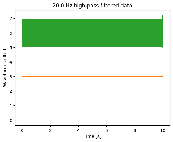
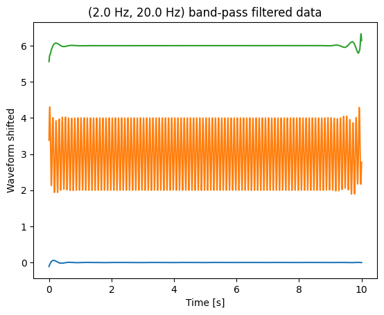
__High-pass __ and __ __ bandpass
beware !
transients !
Filters imply phase shifts. To compensate, combine for- and backward filtering.
Filter first before downsampling (see example).
To inspect a filter, filter a white noise signal and plot PSD.
Take care, transients at start and end of signal
The more parameter you specify, the more difficult is it to design a filter
blue __: __ original signal , sampled at 2500 Hz
red __: __ downsampled to 25 Hz
black __: __ first filtered, then downsampled to 25 Hz
The convolution theorem states that in Fourier space , convolutions are expressed by multiplication of the transformed signal and filter .
If you transform a filter into Fourier space, you can investigate its properties by considering it a ‚mask‘ for your time series representation.
You can use the convolution theorem to perform convolutions efficiently , using FFT.
Example __: __ low __-pass __ filter
__More __ information :
https://davrot.github.io/pytutorial/scipy/scipy.signal_butterworth /
Spectral __ __ analysis
__ __ __ANDA __ tutorial …
Switch
presentations
Wavelet Transform in Python
One can use the pywt module, and requires essentially only two commands for creating a ‚mother wavelet‘ and applying it to the time series of interest:
# The wavelet we want to use...
mother = pywt .ContinuousWavelet ( "cmor1.5-1.0" )
# ...applied with the parameters we want:
complex_spectrum , frequency_axis = pywt . cwt (
data = test_data , scales = wave_scales , wavelet = mother , sampling_period = dt
)
However, working with the wavelet transform requires to think about the scales or frequency bands, their spacing, proper definition of time/frequency resolution, taking care of the cone-of-interest etc…
Full code at: https://davrot.github.io/pytutorial/pywavelet/
__More __ information :
https://davrot.github.io/pytutorial/pywavelet /
__Multidimensional __ representations
Neural recordings often yield a large number of signals xi(t).
Typically, these signals contain a mixture of internal and external sources sj(t). Example __: __ One EEG signal contains the activity of millions of neurons.
__Goal: __ find the neural sources s(t) contained in the signals x(t)
Also:
Assessment of dimensionality of a representation
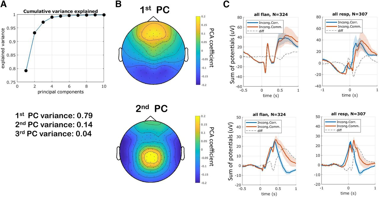
Dimensionality reduction. Get the principal components.
Remove common sources common reference\, line noise\, heartbeat artifacts\, etc\.
…
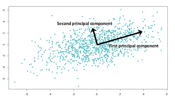
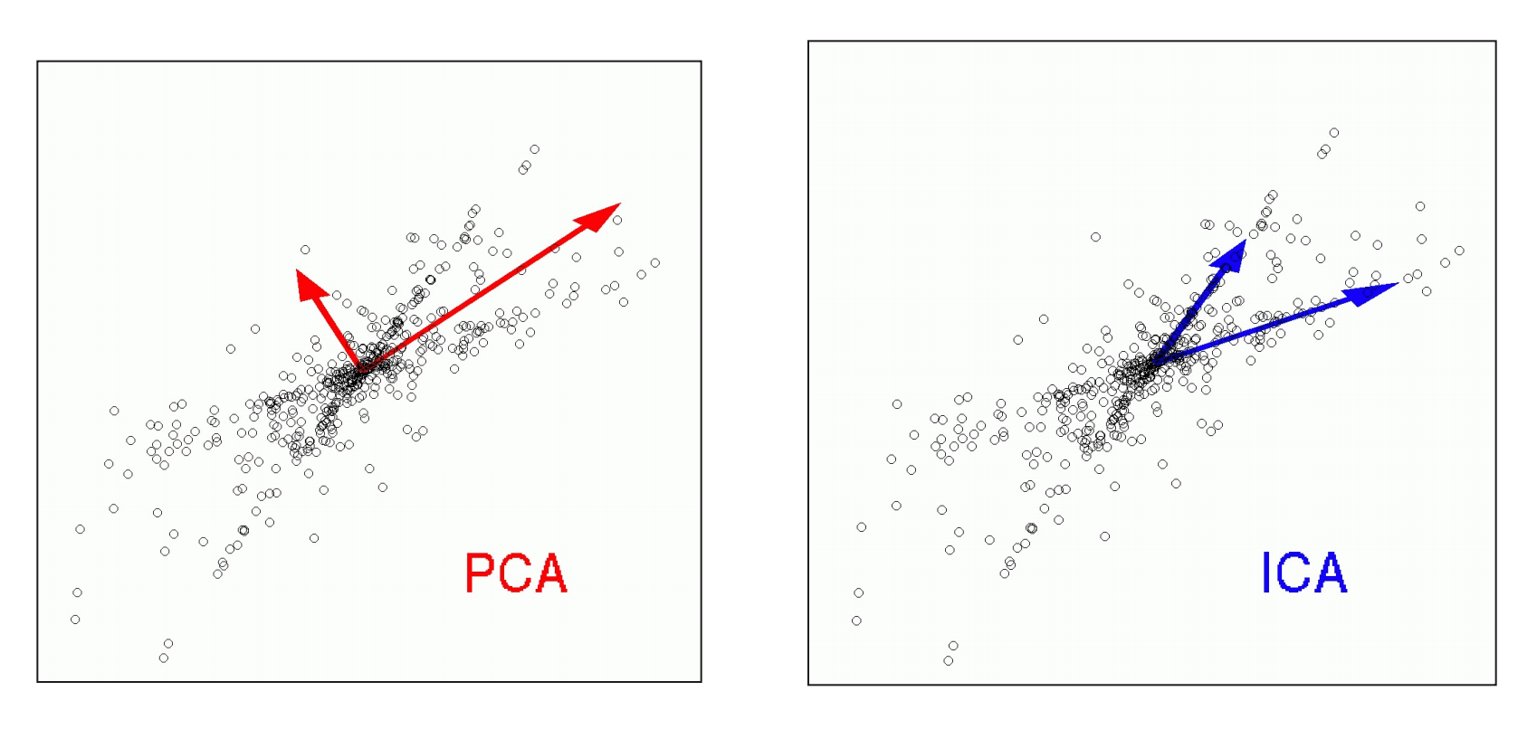
__PCA – __ principal __ __ component __ __ analysis
Find sources which are uncorrelated with each other . Uncorrelated means that the source vectors S will be orthogonal to each other .
PCA finds matrix WPCA such that X is explained by X = S WPCA.
remove mean?
remove std?
W PCA -1 = W PCA T , so S = X W PCA T
Example __: n __ signals __ __ of __ __ duration __ t: __
S: t x n – n source vectors
WPCA: n x n – mixture matrix
X: t x n – n observation vectors
Visualization :
W PCA [k, :] shows how the k- th component contributes to the n observations :
__PCA – __ principal __ __ component __ __ analysis : Python
Use class __ PCA __ from sklearn.decomposition module:
After defining an instance, you can use fit for fitting a transform, and transform for transforming X to S.
fit_transform combines these steps, and inverse_transform __ __ does the transfrom from S to X.
The attribute components _ will contain the PCA transformation components
Components will be sorted with descending </span> <span style="color:#C00000">explained</span> <span style="color:#C00000"> variance .
from sklearn . decomposition import PCA
# transform x to s pca = PCA ()
s = pca . fit_transform ( x )
w_pca = pca . components _
# transform s to x
x_recover = pca. inverse_transform (s)
also_x_recover = s@w_pca
W PCA -1 = W PCA T , so S = X W PCA T
__Take care! __ Instead __ __ of __ X __ __= S __ W PCA __, __ the __ __ transform __ __ is __ also __ often __ __ defined __ __ as __ X‘ __ __= __ W PCA __ S‘. This __ makes __ X‘, S‘ n x t __ instead __ __ of __ t x n __ matrices !
__SVD – Singular Value __ Decomposition
The singular value decomposition decmposes a matrix M into two unitary matrices U and V, and a diagonal matrix ∑: M = U __ __ __∑ V* __
Assumptions are UTU = UUT = I, and VTV = VVT = I with I being the unit matrix.
__Relation __ to __ PCA: __ Consider m denotes ‚time‘ t,and n <=t. Then M are the observations X, V* will be WPCA, and S = U ∑ the uncorrelated principal components, related via: X = S W PCA .
__ICA – __ independent __ __ component __ __ analysis
ICA assumes also a linear mixture of ‚ sources ‘ via X = S W ICA . However, here the goal is to find sources which are statistically independent to each other.
__The ICA __ transform __ __ is __ not __ unique __ __ and __ __ depends __ on __ the __ __ independence __ __ criterion !
remove mean?
remove std?
is STS trivially diagonal?
When might ICA be more appropriate than PCA? Example : __ __
__Independence __ criteria :
minimization of mutual information
maximization of non-Gaussianity
__ICA – __ independent __ __ component __ __ analysis : Python
Use class __ __ FastICA __ __ from sklearn.decomposition module. The usage is very similar to PCA .
from sklearn . decomposition import FastICA
# transform x to s
ica = FastICA ()
s = ica . fit_transform ( x )
w_ica = ica . components _
# transform s to x
x_recover = ica . inverse_transform ( s )
remove mean?
remove std?
is STS trivially diagonal?
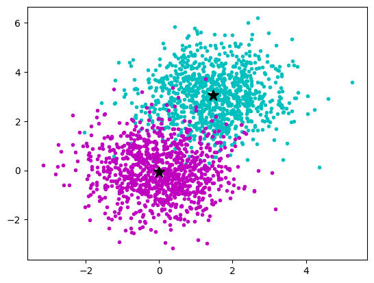
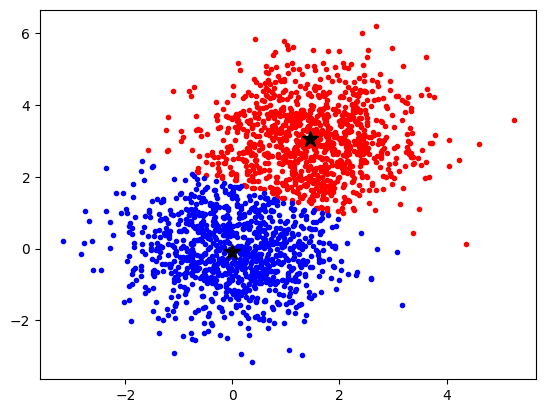
We have multidimensional __ samples __ X and expect that they stem from different ‚classes‘, e.g. spike waveforms where spikes from one particular cell constitute one class. Samples from a particular class should have smaller distance than samples stemming from different classes:
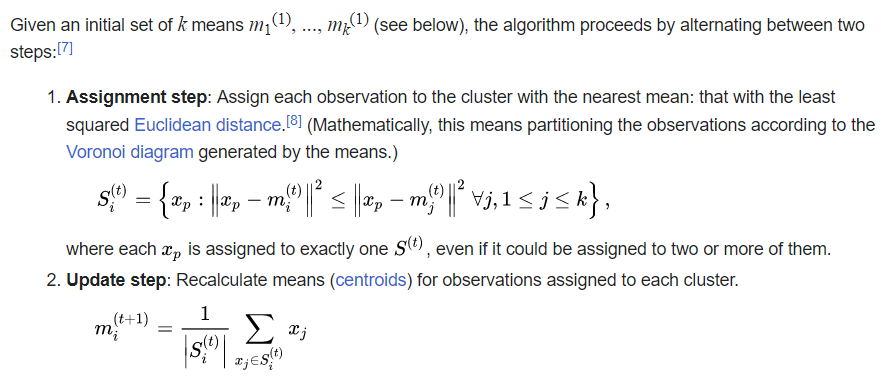
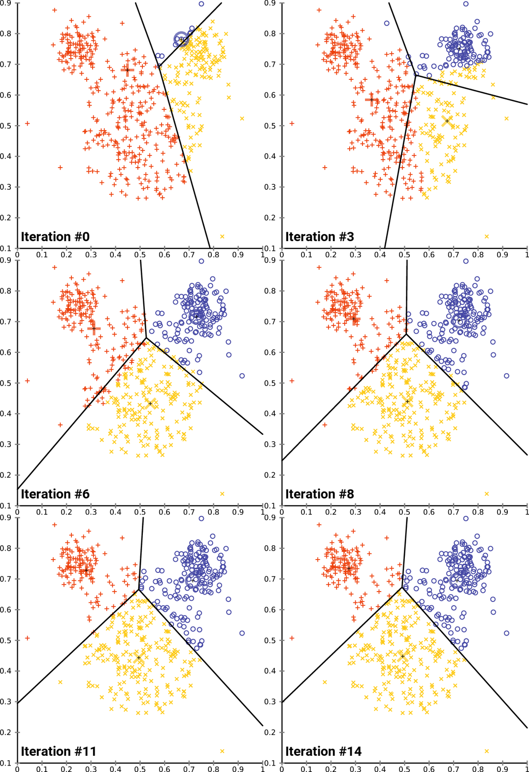
The k- means __ Clustering __ Algorithm
description _ _ and _ _ animation _ _ from _ Wikipedia_
cluster_centers _
The k- means __ Clustering __ Algorithm : Python
__More __ information :
https://davrot.github.io/pytutorial/scikit-learn/overview /
https://davrot.github.io/pytutorial/scikit-learn/pca /
https://davrot.github.io/pytutorial/scikit-learn/fast_ica /
https://davrot.github.io/pytutorial/scikit-learn/kmeans /
Classification __ __ yields __ __ information __ __ about __ __ information __ in __ data …
Receiver-operator- characteristics __ ROC: __ a simple tool for quick inspection for both simple and complex data sets
K- nearest - neighbor __ __ classifier __ __ __kNN__ __: __ easy to implement, suited for a quick inspection
__Support __ vector __ __ machine __ SVM: __ an almost state-of-the-art tool for (non-)linear classification of large data sets. Very useful if you don‘t want to fire up your deep network and NVidia GPU for every almost trivial problem…
Important __: __ For classification , you need a training __ __ data __ __ set , and a test __ __ data __ __ set . Each data set contains a large </span> <span style="color:#FF0000">number</span> <span style="color:#FF0000"> </span> <span style="color:#FF0000">of</span> <span style="color:#FF0000"> samples together with their labels . You are __not __ allowed __ __ to __ __ use __ __ the __ __ test __ __ set __ __ for __ __ training .
__Receiver-Operator __ Characteristics
The situation: one recorded signal r, two potential causes „+“ or „-“:
radio __ __ signal __ r=__ enemy __ __ __plane __ \- __ or __ __ swarm __ __ of __ __ birds __ \+?
How __ __ can __ __ we __ __ distinguish __ __ between __ „+“ __ and __ „-“?__
Simplest estimator: use threshold z, if sample r0 is smaller than z, attribute to „-“, otherwise to „+“
Can we find an optimal z ? Yes, the idea is to plot the true __ positives __ __β__ __ __ against the false __ positives (__ α ) while changing z (ROC curve). Classification accuracy has a maximum / minimum __ __ when __ __ the __ __ rates __ __ of __ __ change __ __ are __ __ equal __ __ ( slope =1) .
__Summary: __ ROC'n'Roll
…it‘s a nice tool for quick inspection how well a scalar variable allows to discriminate between two situations!
What's wrong if the ROC curve is under the diagonal?
Discriminability __: __ difference of means relative to std:
d‘ := (r+-r- )/ σ
k- Nearest - Neighbour __ __ Classifier :
Super-easy to explain, super-easy to implement, super memory consuming!
The x i are samples of the training data set with labels y i .
Every sample from the test data set inside __ __ the __ __ neighborhood __ __ of __ x__ 42 __ __ </span> <span style="color:#0070C0"> __Voronoi__ </span> <span style="color:#0070C0"> __ __ </span> <span style="color:#0070C0"> __cell__ </span> <span style="color:#0070C0"> __ __ gets assigned the label y 42 (k=1)…
…or the majority vote/mixture of the labels __ __ of __ __ the __ k __ nearest __ __ neighbors .
The __ support __ __ vector __ __ machine __ (SVM)
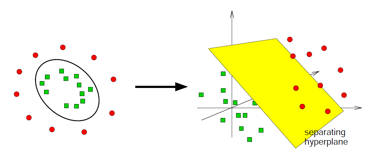
You know how a simple perceptron works lecture Theoretical Neurosciences? The SVM is doing the same thing, but transforms __ __ the __ __ data __ __ into __ a __ higher __-dimensional __ space before it performs a linear __ classification __ __ by __ __ using __ an __ appropriately __ __ placed __ __ separating __ hyperplane :
separating
hyperplane
__Python __ tools __ __ for __ __ elementary __ __ classification __ __ tasks :
ROC and kNN – easy to code on your own (and a good training for you!)…
Learning an SVM is more tricky. scikit-learn provides you with a good tool:
__More __ information :
https://davrot.github.io/pytutorial/numpy/roc /


